


Next: Assignment 10
Up: 22S:194 Statistical Inference II
Previous: Assignment 9
- 9.27
- a.
- The posterior density is
The inverse gamma density is unimodal, so the HPD region is an
interval ![$ [c_1,c_2]$](img553.png) with
with  chosen to have equal density
values and
chosen to have equal density
values and
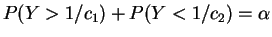 , with
 Gamma
Gamma![$ (n+a, [1/b + \sum x_i]^{-1})$](img556.png) .
.
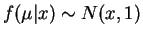
- .b
- The distribution of
 is
Gamma
is
Gamma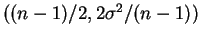 . The resulting posterior density is therefore
As in the previous part, the HPD region is an interval that can be
determined by solving a corresponding set of equations.
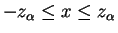
- c.
- The limiting posterior distribution is
IG
![$ ((n-1)/2,[(n-1)s^2]^{-1})$](img563.png) . The limiting HPD region is
an interval with
. The limiting HPD region is
an interval with
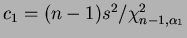 and
and
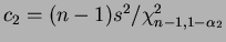 where
where
 and have equal posterior density values.
- 9.33
- a.
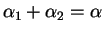
- Since
 for all
  ,
,
For  ,
,
if
 . For
. For  ,
,
if
.
- b.
- For
 ,
,
 .
.
if
and
 .
For
and
.
For
and
 ,
,
as
 .
.
- 10.1
- The mean is
 , so the method of moments
estimator is
, so the method of moments
estimator is
 . By the law of large numbers
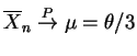 , so
, so
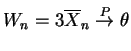 .
.
Next: Assignment 10
Up: 22S:194 Statistical Inference II
Previous: Assignment 9
Luke Tierney
2003-05-04
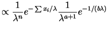
![$\displaystyle = \frac{1}{\lambda^{n+a+1}} e^{-[1/b + \sum x_i]/\lambda}$](img551.png)
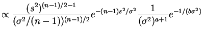
![$\displaystyle \propto \frac{1}{(\sigma^2)^{(n-1)/2 + a + 1}} e^{-[1/b + (n-1)s^2]/\sigma^2}$](img561.png)