 |
||
 |
 |
||
 |
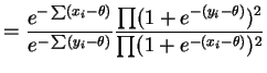
Suppose
![]() . Then for some
. Then for some ![]() one of
one of
![]() is zero and the other is not. So no
is zero and the other is not. So no
![]() exists.
exists.
So
![]() is minimal sufficient.
is minimal sufficient.
 |
 |
|
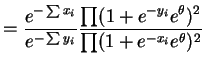 |
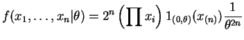
If the ratio is constant in ![]() then the ratio of the two
product terms is constant. These terms are both polnomials of
degree
then the ratio of the two
product terms is constant. These terms are both polnomials of
degree ![]() in
in
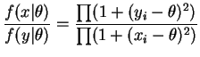
![]() . If two polynomials are equal on an
open subset of the real line then they are equal on the entire
real line. Hence they have the same roots. The roots are
. If two polynomials are equal on an
open subset of the real line then they are equal on the entire
real line. Hence they have the same roots. The roots are
![]() and
and
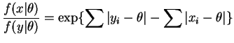
![]() (each of degree 2). If
those sets are equal then the sets of sample values
(each of degree 2). If
those sets are equal then the sets of sample values ![]() and
and
![]() are equal, i.e. the two samples must have the same order
statistics.
are equal, i.e. the two samples must have the same order
statistics.
So the order statistics
![]() are minimal
sufficient.
are minimal
sufficient.
 |
 |
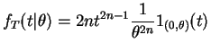
So again the order statistic is minimal sufficient.
 |
||
 |
 |
 |
 |
 |