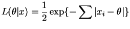
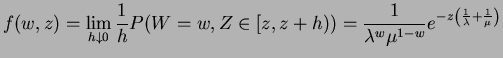
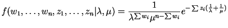
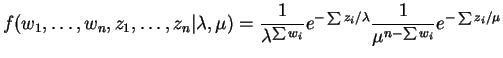
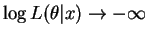
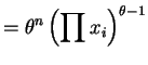
The likelihood and log likelihood are
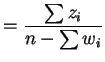
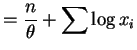
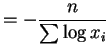
The derivative of the log likelihood and its unique root are
Since
 as
as
 or
or
 and the likelihood
is differentiable on the parameter space this root is a global
maximum.
and the likelihood
is differentiable on the parameter space this root is a global
maximum.
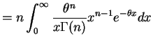
Now
 Exponential
 Gamma
Gamma . So
. So
 Gamma
Gamma . So
. So
and
So
Var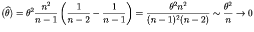 |
|
as
 .
.
![$\displaystyle E_{\theta}[X] = \int_{\theta}^{\infty}x\theta\frac{1}{x^{2}}dx = \theta\int_{\theta}^{\infty}\frac{1}{x}dx = \infty$](img87.png)

![$\displaystyle E\left[-\frac{n}{\sum \log X_{i}}\right]$](img104.png)
![$\displaystyle E\left[\left(\frac{n}{\sum\log X_{i}}\right)^{2}\right] = n^{2}\frac{\Gamma(n-2)}{\Gamma(n)}\theta^{2} = \frac{n^{2}}{(n-1)(n-2)}\theta^{2}$](img107.png)
![$\displaystyle E[X] = \int_{0}^{1}\theta x^{\theta} dx = \frac{\theta}{\theta+1}$](img110.png)