Two Independent Samples

A study on the effect of smoking during pregnancy and lactation on breast milk volume measured the following volumes for samples of 10 smokers and 10 non-smokers:

Volume (g)
Smokers	621	793	593	545	753
	655	895	761	714	598
Non-smokers	947	945	1083	1202	973
	981	930	745	903	899

You can create parallel boxplots of the two samples with the commands Here are parallel boxplots of the samples:

smokers <- c(621, 793, 593, 545, 753, 655, 895, 761, 714, 598) nonsmokers <- c(947, 945, 1083, 1202, 973, 981, 930, 745, 903, 899) boxplot(smokers,nonsmokers,names=c("Smokers","Non-Smokers"))

The summary statistics are obtained with

smokers <- c(621, 793, 593, 545, 753, 655, 895, 761, 714, 598) nonsmokers <- c(947, 945, 1083, 1202, 973, 981, 930, 745, 903, 899) mean(smokers) sd(smokers) mean(nonsmokers) sd(nonsmokers)

They are

		Sample	Sample
	n	mean	SD
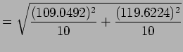
Smokers	10	692.8	109.0492
Non-smokers	10	960.8	119.6224

Estimated difference in means

$$\overline{x}_{\text{\sc{Sm}}} - \overline{x}_{\text{\sc{NonSm}}} = 692.8 - 960.8 = -268$$

is produced by

smokers <- c(621, 793, 593, 545, 753, 655, 895, 761, 714, 598) nonsmokers <- c(947, 945, 1083, 1202, 973, 981, 930, 745, 903, 899) mean(smokers) - mean(nonsmokers)

The standard error

$$= \sqrt{\frac{s_{\text{\sc{Sm}}}^2}{n_{\text{\sc{Sm}}}} + \frac{s_{\text{\sc{NonSm}}}^2}{n_{\text{\sc{NonSm}}}}}$$ SE

$$= \sqrt{\frac{(109.0492)^2}{10} + \frac{(119.6224)^2}{10}}$$

$$= 51.18715$$

is computed by

smokers <- c(621, 793, 593, 545, 753, 655, 895, 761, 714, 598) nonsmokers <- c(947, 945, 1083, 1202, 973, 981, 930, 745, 903, 899) sqrt(sd(smokers)^2/length(smokers) + sd(nonsmokers)^2/length(smokers))

R output for a one-sided test for a significantly lower mean volume among smokers

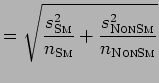         Welch Two Sample t-test 

data:  smokers and nonsmokers 
t = -5.2357, df = 17.848, p-value = 2.872e-05 
alternative hypothesis: true difference in means is less than 0 
95 percent confidence interval:
        NA -179.1973

is computed by

smokers <- c(621, 793, 593, 545, 753, 655, 895, 761, 714, 598) nonsmokers <- c(947, 945, 1083, 1202, 973, 981, 930, 745, 903, 899) t.test(smokers,nonsmokers,alternative="less")

We can also obtain a confidence interval for the difference between the mean volumes for smokers and non-smokers:

smokers <- c(621, 793, 593, 545, 753, 655, 895, 761, 714, 598) nonsmokers <- c(947, 945, 1083, 1202, 973, 981, 930, 745, 903, 899) t.test(smokers,nonsmokers)

         Welch Two Sample t-test 

data:  smokers and nonsmokers 
t = -5.2357, df = 17.848, p-value = 5.743e-05 
alternative hypothesis: true difference in means is not equal to 0 
95 percent confidence interval:
 -375.6059 -160.3941 
sample estimates:
mean of x mean of y 
    692.8     960.8

Try some examples of your own in the work area below.

Work Area

Enter your own commands here; then click the Submit button.